A dive into spatial search algorithms
Searching through millions of points in an instant
I’m obsessed with software performance. One of my main responsibilities at Mapbox is discovering ways to make our mapping platform faster. And when it comes to processing and displaying spatial data at scale, there’s no concept more useful and important than a spatial index.
Spatial indices are a family of algorithms that arrange geometric data for efficient search. For example, doing queries like “return all buildings in this area”, “find 1000 closest gas stations to this point”, and returning results within milliseconds even when searching millions of objects.
Spatial indices form the foundation of databases like PostGIS, which is at the core of our platform. But they’re also immensely useful in many other tasks where performance is critical. In particular, processing telemetry data — e.g. matching millions of GPS speed samples against a road network to generate live traffic data for our navigation service. On the client side, examples include placing labels on a map in real time, and looking up map objects on a mouse hover.
In the last 4 years, I’ve built a bunch of ultra-fast JavaScript libraries for spatial search: rbush, rbush-knn, kdbush, geokdbush (with a few more to come). In this post, I’ll attempt to describe how they work under the hood.
Spatial search problems
Spatial data has two fundamental query types: nearest neighbors and range queries. Both serve as a building block for many geometric and GIS problems.
K nearest neighbors
Given thousands of points, such as city locations, how do we retrieve the closest points to a given query point?
An intuitive way to do this is:
- Calculate the distances from the query point to every other point.
- Sort those points by distance.
- Return the first K items.
This is fine if we have a few hundred points. But if we have millions, these queries will be too slow to use in practice.
Range and radius queries

How do we retrieve all points inside…
- a rectangle? (range query)
- a circle? (radius query)
The naive approach is to loop through all the points. But this will fail if the database is big and gets thousands of queries per second.
How spatial trees work
Solving both problems at scale requires putting the points into a spatial index. Data changes are usually much less frequent than queries, so incurring an initial cost of processing data into an index is a fair price to pay for instant searches afterwards.
Almost all spatial data structures share the same principle to enable efficient search: branch and bound. It means arranging data in a tree-like structure that allows discarding branches at once if they do not fit our search criteria.
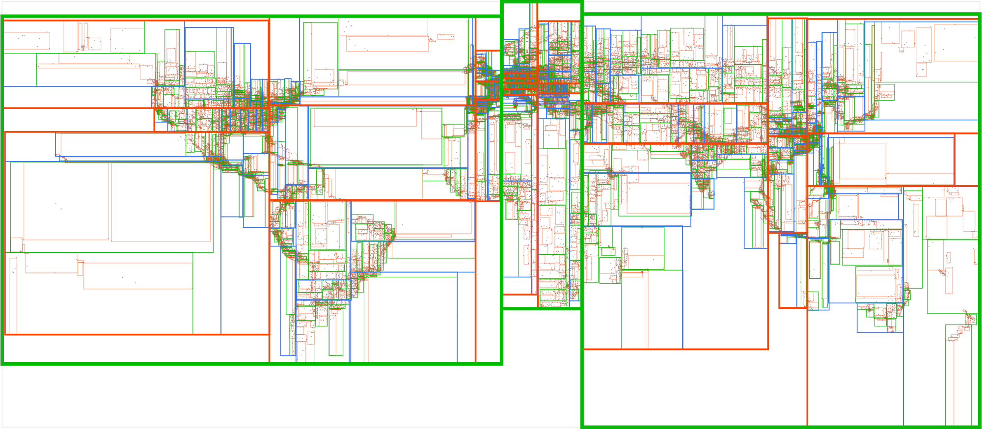
R-tree
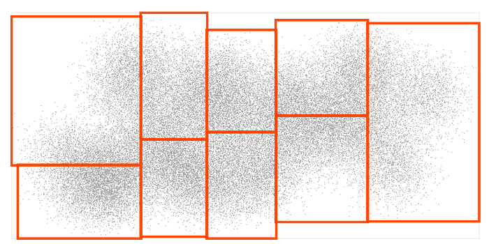
To see how this works, let’s start with a bunch of input points and sort them into 9 rectangular boxes with about the same number of points in each:
Now let’s take each box and sort it into 9 smaller boxes:
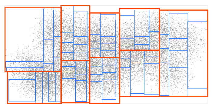
We’ll repeat the same process a few more times until the final boxes contain 9 points at most:
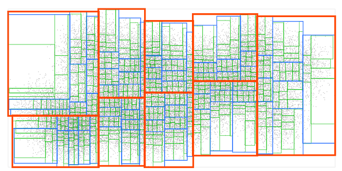
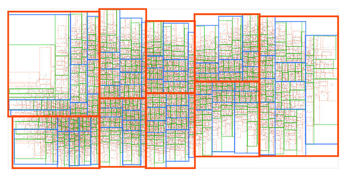
And now we’ve got an R-tree! This is arguably the most common spatial data structure. It’s used by all modern spatial databases and many game engines. R-tree is also implemented in my rbush JS library.
Besides points, R-tree can contain rectangles, which can in turn represent any kinds of geometric objects. It can also extend to 3 or more dimensions. But for simplicity, we’ll talk about 2D points in the rest of the article.
K-d tree
K-d tree is another popular spatial data structure. kdbush, my JS library for static 2D point indices, is based on it. K-d tree is similar to R-tree, but instead of sorting the points into several boxes at each tree level, we sort them into two halves (around a median point) — either left and right, or top and bottom, alternating between x and y split on each level. Like this:

Compared to R-tree, K-d tree can usually only contain points (not rectangles), and doesn’t handle adding and removing points. But it’s much easier to implement, and it’s very fast.
Both R-tree and K-d tree share the principle of partitioning data into axis-aligned tree nodes. So the search algorithms discussed below are the same for both trees.
Range queries in trees
A typical spatial tree looks like this:
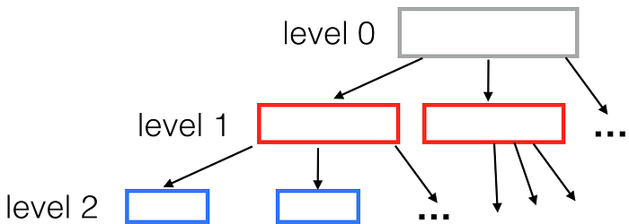
Each node has a fixed number of children (in our R-tree example, 9). How deep is the resulting tree? For one million points, the tree height will equal ceil(log(1000000) / log(9)) = 7.
When performing a range search on such a tree, we can start from the top tree level and drill down, ignoring all the boxes that don’t intersect our query box. For a small query box, this means discarding all but a few boxes at each level of the tree. So getting the results won’t need much more than sixty box comparisons (7 * 9 = 63) instead of a million. Making it ~16000 times faster than a naive loop search in this case.
In academic terms, a range search in an R-tree takes O(K log(N)) time in average (where K is the number of results), compared to O(N) of a linear search. In other words, it’s extremely fast.
We chose 9 as the node size because it’s a good default, but as a rule of thumb, higher value means faster indexing and slower queries, and vice versa.
K nearest neighbors (kNN) queries
Neighbors search is slightly harder. For a particular query point, how do we know which tree nodes to search for the closest points? We could make a radius query, but we don’t know which radius to pick — the closest point could be pretty far away. And doing many radius queries with an increasing radius in hopes of getting some results is inefficient.
To search a spatial tree for nearest neighbors, we’ll take advantage of another neat data structure — a priority queue. It allows keeping an ordered list of items with a very fast way to pull out the “smallest” one. I like to write things from scratch to understand how they work, so here’s the best ever priority queue JS library: tinyqueue.
Let’s take a look at our example R-tree again:
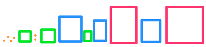
An intuitive observation: when we search a particular set of boxes for K closest points, the boxes that are closer to the query point are more likely to have the points we look for. To use that to our advantage, we start our search at the top level by arranging the biggest boxes into a queue in the order from nearest to farthest:

Next, we “open” the nearest box, removing it from the queue and putting all its children (smaller boxes) back into the queue alongside the bigger ones:

We go on like that, opening the nearest box each time and putting its children back into the queue. When the nearest item removed from the queue is an actual point, it’s guaranteed to be the nearest point. The second point from the top of the queue will be second nearest, and so on.
This comes from the fact that all boxes we didn’t yet open only contain points that are farther than the distance to this box, so any points we pull from the queue will be nearer than points in any remaining boxes:
If our spatial tree is well balanced (meaning the branches are approximately the same size), we’ll only have to deal with a handful of boxes — leaving all the rest unopened during the search. This makes this algorithm extremely fast.
For rbush, it’s implemented in rbush-knn module. For geographic points, I recently released another kNN library — geokdbush, which gracefully handles curvature of the Earth and date line wrapping. It deserves a separate article — it was the first time I ever applied calculus at work.
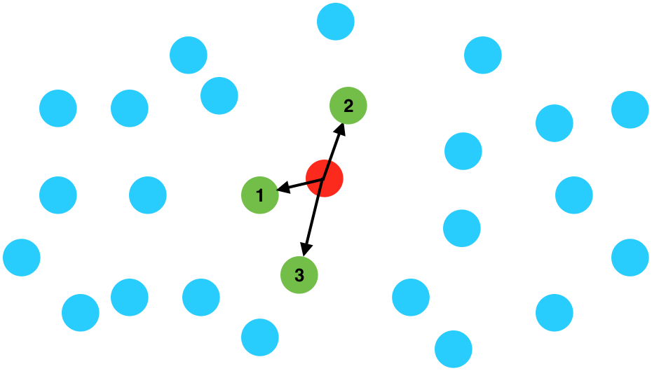
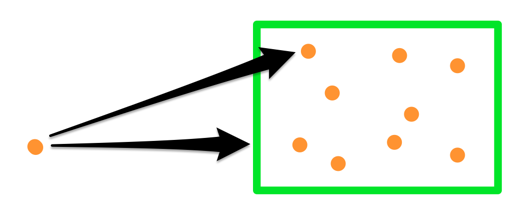
Custom kNN distance metrics
This box-unpacking approach is quite flexible, and works for other distance types besides point-to-point distances. The algorithm relies on a defined lower bound of distances between the query and all objects inside a box. If we can define this lower bound for a custom metric, we can use the same algorithm for it.
This means we can, for example, change the algorithm to search K points closest to a line segment (instead of a point):
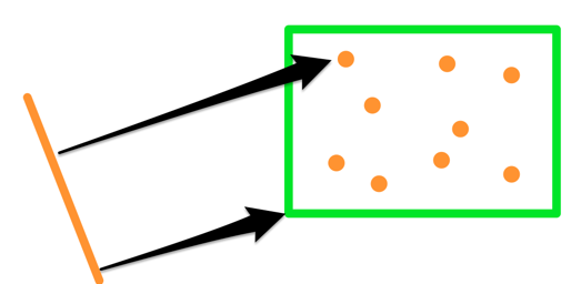
The only modification to the algorithm we need is replacing point-to-point and point-to-box distance calculations with segment-to-point and segment-to-box distances.
In particular, this came in handy when I built Concaveman, a fast 2D concave hull library in JS. It takes a bunch of points and generates an outline like this:
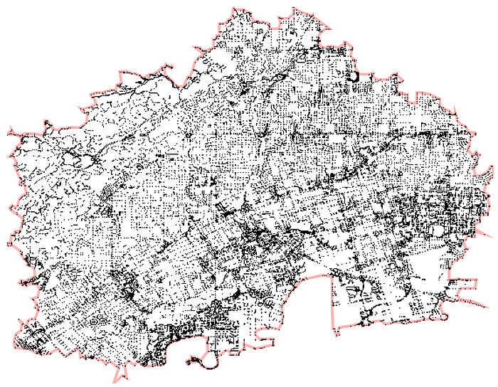
The algorithm starts with a convex hull (which is fast to calculate), and then flexes its segments inward by connecting them through one of the closest points:
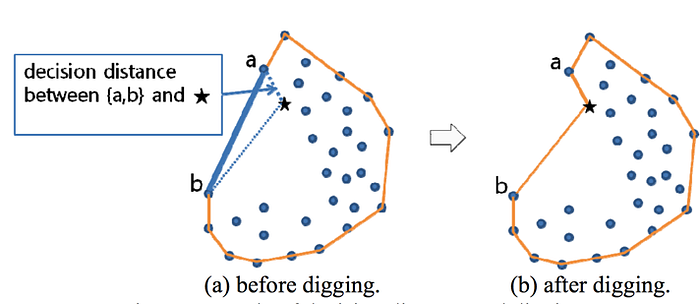
Here’s a quote from the paper on that operation:
In our proposed concave hull algorithm, finding nearest inside points — these are candidates of target spots for digging — from boundary edges is a time-consuming process. Developing a more efficient method for this process is a future research topic.
Which I advanced, by a lucky coincidence! Indexing the points and performing “closest points to a segment” queries made the algorithm very fast.
To be continued
In future articles in the series, I’ll cover extending the kNN algorithm to geographic objects, and go into detail on tree packing algorithms (how to sort points into “boxes” optimally).
Thanks for reading! Feel free to comment and ask questions, and stay tuned for more. Play with our awesome SDKs, and if you’re fired up about hard engineering challenges and maps, check out our job openings.